Research Article - Onkologia i Radioterapia ( 2023) Volume 17, Issue 9
A comparison of dose distribution between Scan2MCNP and CT2MCNP programs for brachytherapy of brain tumours
Hadi Nasrollahi1*, Mohsen Hasani2, Hasan Ali Nedaei2 and Hamideh Naderi32Department of Radiotherapy Physics, Cancer Research Centre, Cancer Institute, Tehran University of Medical Sciences, Tehran, Iran
3Department of Medical Physics, Qom University of Medical Sciences, Qom, Iran
Hadi Nasrollahi, Radiation Oncology Division, Turkish Hospital, Karbala, Iraq, Email: hnasrollahi@muq.ac.ir
Received: 31-Jul-2023, Manuscript No. OAR-23-108580; Accepted: 08-Sep-2023, Pre QC No. OAR-23-108580 (PQ); Editor assigned: 03-Aug-2023, Pre QC No. OAR-23-108580 (PQ); Reviewed: 25-Aug-2023, QC No. OAR-23-108580 (Q); Revised: 04-Sep-2023, Manuscript No. OAR-23-108580 (R); Published: 15-Sep-2023
Abstract
Introduction: The use of Monte Carlo simulation methods is assumed to be one of the most accurate methods for calculation of dose distribution in a patient's body. Two pieces of software in MCNP code, which are applied for body simulation, are Scan2MCNP and CT2MCNP that operate based on the intensity of DICOM colour images and CT numbers respectively. Therefore, dose distribution obtained by these two methods is predicted to be different. The aim of this study is to evaluate dosage differences calculated by Scan2MCNP and CT2MCNP to simulate of low energy radioactive sources for brachytherapy of brain tumours. Material and methods: In this study, 125I (Model IR-Seed2) source manufactured by Iran was simulated by MCNPX code and then the accuracy of simulation was evaluated. Simulation of 125I implantation in brain was performed using Scan2MCNP and CT2MCNP programs. Comparison of the sources' implant time, isodose curves and Dose Volume Histograms (DVH) between these two pieces of software was performed. Results: The simulations showed that Scan2MCNP software, due to using higher density materials and more attenuation, predicted lower dose value compared to CT2MCNP. Conclusion: The results showed that Scan2MCNP software, because of using colour image intensities revealed in simulation of soft tissues and bone inhomogeneity, led to about 10% and 25% error, respectively.
Keywords
monte carlo, ct2mcnp, scan2mcnp, 125i source, brain tumour, brachytherapy
Introduction
Radiotherapy uses ionizing radiation to kill cancer cells. It aims to deliver effective doses to tumours while minimizing harm to healthy tissues. Prior to treatment, creating a suitable plan and accurately predicting dose distribution is essential [1]. Commercial treatment planning systems, due to the use of mathematical models for dosimetric calculations, have limitations that cause differences between predicted dose distribution in these systems and actual dose distribution in a patient's body. Due to the dosimetric limitations of Task Group 43 (TG-43U1) report of the American Association of Physicists in Medicine (AAPM), these differences are more probable in brachytherapy planning systems that use TG-43 protocol for dosimetric calculations [2-4]. The methods of Monte Carlo calculations and the use of codes such as FLUKA, MCNPX, GEANT4 and PENELOPE are assumed to be the most accurate methods for dosimetry and determination of dose distribution of ionizing radiation beams in a patient's body. However, the speed of calculations and difficulty of body simulation cause limitations in applying Monte Carlo techniques. One of the methods that is used for simulation of the anatomical structures of patients in MCNP code is Scan2MCNP software. This program takes the DICOM (Digital Imaging and Communications in Medicine) images of a patient and selects the materials used in simulation by image color intensities, while CT2MCNP uses CT numbers for material simulation in MCNP code [5]. The basis of CT2MCNP and Scan2MCNP programs are to read the CT files of the patient and ensure that they are three-dimensional, while assigning a substance with a specific composition and density to each voxel, reducing the number of cells by combining the adjacent cells with the same square mesh, assigning the new substances and densities to new cells, and combining adjacent cells with larger cells (if they all consist of a single substance). Therefore, they have errors in calculation relative to the clinical state and TG-43 [6]. The purpose of this study is to use CT2MCNP and Scan2MCNP programs to simulate 125I sources used for the treatment of brain tumours and also evaluate the differences between predicted dose distribution and these two pieces of software.
Methods
In this study, we first studied the dose distributions of 125I source manufactured by Iran of model IR-Seed2 125I and compared it with the dose distributions of the 125I standard sources of models 6702 and 6711. To evaluate the validity of the simulations, we used Perspex phantom and TLD (Thermoluminescent dosimeter). In the following, treatment planning of brain tumours by 125I source was performed using by Scan2MCNP and CT2MCNP programs in the MCNPX code for different-source allocation. These two pieces of software use different methods, and they are used for the definition of geometry and different ma terials in Monte Carlo simulation.
IR-Seed 2 125I source
IR-Seed2 125I source consists of a cylindrical titanium capsule (with 48 mm long and 0.8 mm diameter) and two caps at the opposite ends (0.65 mm thick). The internal diameter of the source is 0.7 mm and it has six microspheres resin beads with 0.5 mm diameter and percentage weight composition of: H 8%; C 90%; N 0.3%; Cl 0.7%; I 1% as well as 125I superficially covers these beads. The activities of the outermost beads were 2.2 m Ci, the next two beads were 2.3 mCi, and the remaining two beads (closest to the center of the source) were 1.7 m Ci [7]. When we used it, the overall activity of the source was 1.85m Ci and phantom radiation with TLDs was done for 48 hours.
This s ource w as s imulated in the centre of a Perspex sphere with 10 cm diameter. Absorbed dose values were taken in the perpendicular direction of the source axis using a square mesh. Meshing was performed as cubic voxels with 0.8 mm dimensions covering entirely the space around the source up to 7 cm distance. Figure shows the simulation of 125I source by MCNPX code (Figure 1).

Figure 1: The simulation of 125I source by MCNPX code
Thermoluminescent dosimetry
The results of the source simulation were compared with the results of the source dosimetry with thermoluminescent dosimeters by GR-207A TLDs. These TLDs are chip forms with 4.5 mm diameter and 0.8 mm thickness that show linear response in 10-6 12 Gy [8]. These kind of thermoluminescent dosimeters are also known as 7-LiF: Mg, Cu, P (Fimel, Vélizy, France). These chips annealing was performed according to the manufacturer's recommendation (240°C, 10 min) [9]. Although utilization of average data of several TLD chips can decline statistical fluctuations, it may cause some variations, based on their mass and physical geometries differences. Consequently, to avoid these effects, ECC (Element Correction Coefficient) was employed by calculating the ratio of the measured responses of each chip to the overall average responses to the same exposure. These seven calibrated GR-207A TLDs were subjected to irradiation of sources for 48 hours. The activity of 125I source was 1.85m Ci. After irradiation, the TLDs were read by an LTM TLD reader (Fimel, Vélizy, France) and the dose received was calculated.
Importing Images into MCNP
DICOM image:
DICOM format files consist of two binary files: an image file with the extension “img” that contains the voxel raw data and a header file with the extension “hdr” that includes the metadata, such as the number of pixels in x, y, and z directions, voxel size, and data type [10]. During each CT-scan, many x-ray photons are transmitted through each voxel and the intensity of the transmitted x-ray is measured. By considering the magnitude of attenuation in each voxel, a numerical value is allocated to the voxel. This value is compared to attenuation in water and displayed with a scale which is named Hounsfield Unit. In fact, each CT image is a two dimensional array of a Hounsfield Unit. The range of these numbers are between -1000 to +1000. The Hounsfield Unit of water is zero. Each number represents a level of grayscale. For example, bone with +1000 HU is represented by white colour and air with -1000 HU is shown by black colour. Other numbers are displayed as grayscale level between white and black [11].
In this study, CT images of a brain tumour of the patient were used for body simulation and 3D Scan2MCNP software was used for brain simulation. In order to simulate the head of a patient with a brain tumour, 41 CT images of the patient were used. The tumour size in this patient is a circle with approximate radius of 1.6 cm and approximate volume of 17.5 cm3. Figure shows CT and MR images of this patient (Figure 2).

Figure 2: CT and MR images of patient with brain tumour
Scan2MCNP software
Importing patient's data to MCNP program is one of the most important stages in Monte Carlo-based simulations and Scan2MCNP software can convert DICOM images from MRI and CT imaging systems to entrance file for MCNP code. This software has a library of different materials with their densities, such as a number of gases, liquids, metals and materials of body tissues like bone, soft bone, soft tissue, lung, etc. This software uses intensity in colour images to assign different materials in simulation. Each image has grayscale numbers ranging from 0 to 256. For example, the white pixels have colour intensity of 256 and are related to bone; the black pixels have colour intensity of 0 and are related to air. Other pixels with various colour intensities between 0 and 256 belong to other materials [12].
The number of cells simulated in the MCNPX after using the Crop command and meshing in the Scan2MCNP program, which considers the area of tumour and its surroundings, is equal to 243089. Each cell has dimensions of 0.094 cm × 0.094 cm × 0.2 cm, which is appropriate for studies on low energy brachytherapy Figure 3 shows the brain simulation of the patient in MCNPX code using Scan2MCNP software (Figure 3).

Figure 3: The simulation of brain using Scan2MCNP code
CT2MCNP software
CT2MCNP software was designed to read and simulate CT images of a patient's body. This software is approximately similar to Scan2MCNP, but only uses HU instead of colour intensities of each voxel for assigning materials in MCNP code. In this software, the data from CT images are converted into an input in MCNP code in several stages:
• The CT files of a patient are interpreted to be sure that the files are 3D.
• A material with specific composition and density is assigned to each voxel.
• The number of cells is reduced via compilation of adjacent cells with equal quadratic mesh, and new materials and densities are considered for new cells.
• Adjacent cells and larger cells are combined if all of them are made up of one material [13, 14].
Figure 4 shows part of brain simulation of a patient by CT2MCNP software (Figure 4). After simulation of the brain region by CT2MCNP, 125I sources were simulated in tumour and all other stages of simulation were similar to Scan2MCNP software in terms of the number of sources, activities and source locations.

Figure 4: The simulation of brain of patient with CT2MCNP software
By using MCNPX code, the time of source implants, isodose curves, DVHs and absorbed dose to different areas of tumour for different source implants were obtained and compared to results from Scan2MCNP software.
Monte carlo calculations
In this investigation, the simulation was performed by The Los Alamos National Laboratory (LANL) Monte Carlo N-Particle radiation transport code MCNPX 2.7.0. There are several various types of tally to calculate different physical properties in the MCNPX. The use of mesh tally method is one of the most applicable methods for reducing the entrance data in MCNP code in programs with large numbers of cells. Therefore, MCNP simulation was run by the third type of mesh tally for a number of 1010 particles. The average of absorbed dose in each voxel was obtained in a case whose activity of each source was 3 m Ci. Its output is in MeV/cm3 , which should be divided into density to convert it into the absorbed dose. MCNPX employs 125I photon spectrum extracted from ICRU-38 [15]. The energy cut-off δ=5 keV was considered in terms of the titanium characteristic X-ray production [16]. In order to evaluate the validity of simulation performed in the MCNPX, absorbed dose was calculated to water in Perspex to provide comparable data with the TLD measurements.
The code written for 1010 particle was executed, so that the average program error in the code for all cells was lower than 5%. The isodose curves of code output were depicted in MATLAB software version 7.9.0 (R2009b) using reshape, resize, imrotate, and rcond commands, and cast on patient’s MR images.
Phantom
To assess the agreement between simulation performed in the MCNP and TLD measurements, a phantom made of Perspex with a mass density of 1.19 g/cm3 , composition of H 8%; C 60%; O 32% and dimensions of 30 cm3 × 30 cm3 × 1.5 cm3 was produced [17]. As shown in Figure, a groove was made in the centres of the phantom for placement of source, as well as grooves at 0.5 cm, 1 cm, 1.5 cm, 2 cm, 3 cm, 4 cm and 5 cm distances in the perpendicular direction of source axis for placing TLDs were devised (Figure 5). Simulation of 125I source with MCNPX code was done in a phantom made of Perspex with dimensions 11 cm3 × 11 cm3 × 11 cm3 quite similar to practical irradiation mode and the structure of this simulation is based on lattice.

Figure 5: The phantom used for the 125I source dosimetry
Placement of sources in the tumour
Implantation of a single source in the head of the patient with brain tumour is the common method for treatment of this disease. Hence, apart from the size, shape and volume of the tumour, the implant of 125I source was performed in the simulation, the first of which was simulated in the centre and the latter 2, 4 and 8 sources in tumour region. The distance of source centers was 1 cm from each other. Figure shows the simulation of two sources implanted in tumour in the MCNPX code (Figure 6).

Figure 6: Two sources implanted in tumour in the MCNPX code
Treatment time calculation
In brachytherapy, source allocation of time and space determine the delivered doses. For this reason, the medical information of a low grade patient with tumour volumes of 17 cm3 , including 6000 cGy doses at the border of the tumour, was identified by an oncologist and then, given that the source's activity is equal to 3 mCi, treatment time was obtained by calculating the MCNP data. With the dose rate and prescriptive dose, treatment time was calculated according to Equation 2. In the calculation of the output of the code in the mesh tally method, the output is obtained for a particle, this value converts to delivered dose using Equation 1, and the treatment time is obtained using the Equation 2.
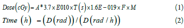
A represents the activity in mCi unit, T is the duration of the irradiation of the source, F is the value obtained from the MCNPX code and M represents the absorption coefficient of the radioactive material, which is 1.47 for 125I [18].
Results
TLD Calibration
For TLDs calibration with multiply ECC coefficient for each TLD to the amount of reading could reduce the effect of random variations and get to a constant value. Table indicates the correction coefficients that were calculated for each TLD and Figure shows the diagram of TLD's calibration curve in 120 kVp (Table 1 and Figure 7).
Tab. 1. The ECC correction coefficients for TLD calibration
| TLD No. | ECC | TLD No. | ECC |
|---|---|---|---|
| 1 | 0.964 | 10 | 1.021 |
| 2 | 0.999 | 11 | 1.019 |
| 3 | 0.972 | 12 | 0.993 |
| 4 | 1.002 | 13 | 0.978 |
| 5 | 1.001 | 14 | 0.997 |
| 6 | 0.992 | 15 | 1.015 |
| 7 | 1.01 | 16 | 1.022 |
| 8 | 0.976 | 17 | 1.022 |
| 9 | 1.024 | 18 | 1.011 |

Figure 7: TLDs calibration curve with a 120 kVp X-ray beam
Simulation evaluation
The acquired results of simulation were compared to the results of dosimetry of one 125I source by GR-207A TLD in a Perspex phantom. The results showed that there was an acceptable agreement (average error in code output <%5) between practical data and the results of simulation by mesh tally method. Table shows the comparison between results of TLD dosimetry and simulation by MCNPX code in source axis direction at different distances (Table 2).
Tab. 2. Comparison between results of TLD dosimetry and simulation in MCNPX
| Distance from Center of Source (cm) | MCNPX Calculated (cGy) | TLD Measured (cGy) | Difference TLD and MCNPX (%) |
|---|---|---|---|
| 0.5 | 406.64 | 433.7 | 2.6 |
| 1 | 93.69 | 100.02 | 2.9 |
| 1.5 | 40.09 | 42.63 | 3.1 |
| 2 | 20.61 | 22.3 | 3 |
| 3 | 5.39 | 6.06 | 3.2 |
| 4 | 2.02 | 2.21 | 4.4 |
| 5 | 1.16 | 1.3 | 5 |
The results were obtained by 1, 2, 4 and 8 source implants in tumour using Scan2MCNP and CT2MCNP programs. Table shows the comparison of the time of source implants and volume amounts that received a dose of 60 Gy in the total treatment time (Table 3). As these data show, CT2MCNP predicts higher doses compared to Scan2MCNP.
Tab. 3. Comparison of the results from Scan2MCNP and CT2MCNP softwares in term of time of implant and the brain volume that received a dose of 60 Gy in different source implants
| Number of | Scan2MCNP | CT2MCNP | ||||
|---|---|---|---|---|---|---|
| Sources | ||||||
|
|
(Days) | (cm3) | (cm3) | (Days) | (cm3) | (cm3) |
| 1 | 550 | 44.2 | 17.2 | 440 | 46 | 17.2 |
| 2 | 132 | 26.82 | 17.2 | 113 | 28.01 | 17.2 |
| 4 | 51.5 | 22.42 | 17.2 | 46 | 24.2 | 17.2 |
| 8 | 22.3 | 17.68 | 17.2 | 20 | 20.05 | 17.2 |
Based on Equation 2, the time required to reach the 6000 cGy dose to the tumour border using Scan2MCNP for one source was calculated 550 days. Also, the delivered dose reaching different parts of the tumour was calculated based on the isodose curves and the total duration of the sources planting during the treatment, which is presented in (Table 3).
Table 3 Comparison of the results from Scan2MCNP and CT2MCNP softwares in term of time of implant and the brain volume that received a dose of 60 Gy in different source implants.
Isodose curves from simulation of various sources by Scan2MCNP and CT2MCNP were obtained using MATLAB software. Figure represents the comparison of isodose curves for 1, 2, 4 and 8 source implants (Figure 8).

Figure 8: Comparison of isodose curves from Scan2MCNP and CT2MCNP softwareâ??s for placing of A. one source, B. two sources, C. four sources and D. eight
In order to compare the isodose curves of the Scan2MCNP and CT2MCNP, these isodose curves of the two methods were obtained for a special period of time and were thrown onto an image. Figure shows the comparison among the isodose curves in the allocation of 1, 2, 4, and 8 number of sources (Figure 8). As the figure shows, CT2MCNP predicted higher dosage than Scan2MCNP. For example, in the presence of one source, in the grey part of the brain, differences of 15% in the dose of 600 Gy, 12.5% in the dose of 200 Gy, 11% in the dose of 100 Gy and 5% in the dose of 60 Gy were observed. In the heterogeneous part including the skull bone, there was a higher dose difference, so that the Scan2MCNP software could not predict the dose of 100 Gy in the bone. In the dose of 60 Gy, within the bone, the CT2MCNP software predicted a 24% higher dose than Scan2MCNP. The differences between isodose curves of different source implants are mentioned in (Table 4).
Tab. 4. The difference (%) between isodose curves of various source implants from Scan2MCNP and CT2MCNP softwareâ??s
| Number of Sources | 60 | 100 | 120 | 150 | 200 | 400 | 600 | 800 |
|---|---|---|---|---|---|---|---|---|
| 1 | 5 | 11 | - | - | 12.5 | - | 15 | - |
| 2 | 7 | - | - | 9 | - | 13 | - | 14 |
| 4 | 8 | - | 9 | - | - | 11 | - | |
| 8 | 8.5 | - | 13 | - | 15.5 | - | - | - |
Table lists magnitude of absorbed dose (Gy) and density of each voxel in various distances around the sources for four source implants from both simulationsly. Figure depicts a comparison of DVHs in four source implants by these pieces of software (Table 5) (Figure 9).
Tab. 5. A Comparison of absorbed dose (Gy) around the tumour by Scan2MCNP and CT2MCNP programs
| Distance from the Center of Tumor | Scan2MCNP | CT2MCNP | Difference | ||
|---|---|---|---|---|---|
| (cm) | Dose (Gy) | Density (g/cm3) | Dose (Gy) | Density (g/cm3) | (%) |
| 1 | 181.3 | 1.04 | 203.71 | 1.06 | 11.21 |
| 1.5 | 73.51 | 1.04 | 80.34 | 1 | 8.53 |
| 2 | 33.55 | 1.04 | 36.08 | 0.97 | 7.02 |
| 2.5 | 15.8 | 1.04 | 16.99 | 0.99 | 7.13 |
| 3 | 9.38 | 1.04 | 9.83 | 1 | 4.51 |
| In Bone Tissue | 84.68 | 1.41 | 116.02 | 1.56 | 27.03 |

Figure 9: Comparison of DVHs for four sources implants from Scan2MCNP and CT2MCNP
Discussion
In this study, IR-Seed2 125I source manufactured by Iran was simulated by MCNPX code and then the accuracy of simulation was evaluated. Simulation of 125I implantation in brain was performed using Scan2MCNP and CT2MCNP programs. The comparison of source implant time, isodose curves and Dose Volume Histograms (DVH) between these two pieces of software were performed.
As shown in Table, the results of study for the volume receives a dose of 60 Gy impling that implantation of one source in tumour region not only eradicates cells in a volume equivalent to 17 cm3 but also destroys 1.7 times more of the tumour volume of surrounding tissues (Table 3). Thus, such a great volume in a critical organ like brain is considerable. As the isodose curves show, bone inhomogeneity represents higher dosage than soft tissue. It is due to higher effective atomic number of bone (Zeff=8.9) compared to soft tissue (Zeff=6.2). It leads to an increase in photoelectric absorption effect that is directly proportional to the third power of atomic number (Z3). The average density of brain tissue in Scan2MCNP software is 1.04 g/cm3 , while this value in CT2MCNP software is 0.98 g/cm3 . The higher density in Scan2MCNP software leads to more attenuation in soft tissues, so lower photons reach bone inhomogeneity compared to CT2MCNP software. As a result, this software predicts higher dose than Scan2MCNP software. For example, in one source implantation, the difference between 60 Gy isodose curves in these two pieces of software is about 25%. Moreover, Scan2MCNP software is not able to predict 100 Gy isodose curves, while CT2MCNP software can estimate this value. The differences between 60 Gy isodose curves in 2-source implants are 23% and in 4- and 8-source implants, the dose is not predictable by Scan2MCNP software as it is predictable in CT2MCNP software. More attenuation in Scan2MCNP software leads to a difference in dose and this difference is more significant at areas around the source and due to reduction in photon flux, these differences are lower when the source distance increases. For example, in the situation of one-source implantation, 15%, 12.5%, 11%, and 5% differences were observed in gray matter for absorbed doses of 600 Gy, 200 Gy, 100 Gy and 60 Gy, respectively. The results of the simulations by Scan2MCNP show that it uses color images intensity for definition of various materials of body, and takes the density of soft tissues identically; since this density is higher in the simulation by CT2MCNP, Scan2MCNP software forecasts longer time of radioactive source implants. Comparing these programs showed that using Scan2 MCNP software causes about 10% discrepancy in dose distribution around the sources, while the amount of discrepancy in inhomogeneity such as bone is about 25%.
Significant differences in the delivered dose were reported between TG-43 calculations and the model-based dose calculations with phantoms containing non-water materials. For instance, Mark J. Rivard and his colleagues studied the treatment of ocular melanoma with sources of 103Pd and 125I. They compared the distribution of doses obtained in Pinnaclae v8.odp1, Brachy Vision v8.1 and Plaque simulator treatment systems with dose distribution obtained from MCNP5 and EGSnrc codes. All of the treatment planning systems used in this study have utilized the TG43 method. The results have reported that when a homogeneous media such as water is used in Monte Carlo systems, the difference less than 2% is observed, contrasted to heterogeneous materials such as body tissues, in which the difference about 37% is observed compared with commercial treatment planning systems. As well, it was observed that if the prescription dose was 85 Gy in depth of 5 mm, this dose would be calculated in Monte Carlo systems as about 67 Gy [19]. In another study, Burns and his colleagues also studied the inhomogeneity of tissues in lung brachytherapy by 125I source. In their study, a phantom of the chest with the density of its constituents was realistically simulated. EGSnrc code was used in this method and the delivered dose of different tissues such as bone, lung and soft tissues was calculated and DVH curves were plotted and then the results were compared with the commercial treatment planning programs used by the TG-43 method. The r esults o f t his c omparison s howed significant differences. A difference of 17% for 10 mm around the target volume of treatment (PTV10), 26% in total dose volume (V100) and 20% in the 90% isodose curve (D90) observed in the average absorbed dose. calculated dose in Monte Carlo method, 20 Gy was higher than TG-43 method, which was about 20% of prescriptive dose. It was also observed that there was a significant d ifference between the isodose curves in these two methods, in which the difference in soft tissues was more than lung tissue [20]. Another study by Hulian zhang and his colleagues at the Kentucky University's Center was conducted in 2005. They showed that the prostatic dose in the Monte Carlo method and the dose calculating algorithms in the commercial treatment planning system were approximately 100% in agreement, but the DVH curves for the Variseed treatment planning system averaged 29% higher doses for the same isodose curve. These differences were due to the fact that, firstly, the Variseed treatment planning system uses a point source approximation to calculate the dose, and secondly, it does not take into account the effects of spontaneous self-absorption [21]. Due to the limitations mentioned in the dose calculation algorithms, there is a significant difference between the predicted dose of these algorithms and the actual delivered dose in the patient. This difference in dose in the area of the head, where many sensitive organs are located, is more important and can have a great impact on the quality and survival of patients. Therefore, the need for a treatment planning system that is able to predict the accurate dose distribution in the patient before starting treatment is necessary.
Conclusion
The comparison of dose distribution between Scan2MCNP and CT2MCNP Programs for IR-Seed2 125I brachytherapy of brain tumours has been performed. A complete set of calculations was presented for source implant time, isodose curves, and DVHs. The simulations showed that Scan2MCNP software, due to using higher density materials and more attenuation, predicted lower dose value compared to CT2MCNP as well as because of using colour image intensities revealed in simulation of soft tissues and bone inhomogeneity, led to about 10% and 25% error, respectively.
Conflicts of Interest
There are no conflicts of interest. The authors report no proprietary or commercial interest in any product mentioned or concept discussed in this article. The authors alone are responsible for the content and writing of this article.
References
- Khan, Faiz M, John P. Gibbons. Khan's the physics of radiation therapy. Lippincott Williams Wilkins, 2014.
- Mishra S, Deshpande S, Pathan MS, Selvam TP. DICOM CT-based Monte Carlo dose calculations for prostate permanent implant using 125I. Radiat Phys Chem. 2023;210.
- Williamson JF, Butler W, DeWerd LA, Saiful Huq M, Ibbott GS, et al. Recommendations of the American Association of Physicists in Medicine regarding the Impact of Implementing the 2004 Task Group 43 Report on Dose Specification for and Interstitial Brachytherapy. Med phys. 2005;32(5):1424-1439.
- Poher A, Berumen F, Ma Y, Perl J, Beaulieu L. Validation of the TOPAS Monte Carlo toolkit for LDR brachytherapy simulations. Physica Medica. 2023;107.
- Boia LS, Silva AX, Facure A, Cardoso SC, Rosa L. Methodology for converting CT medical images to MCNP input using the Scan2MCNP system.
- González Martí M. Assessment and further development of programs for medical therapy using fussion neutrons.
- Sheikholeslami S, Nedaie HA, Sadeghi M, Pourbeigy H, Shahzadi S. Monte Carlo calculations and experimental measurements of the TGâ?43U1â?recommended dosimetric parameters of 125I (Model IRâ?Seed2) brachytherapy source. J Appl Clin Med Phys. 2016;17:430-441.
- Furetta C. Handbook of thermoluminescence. World Sci; 2010.
- Salehi Z, Yusoff AL. The absorbed dose in femur exposed to diagnostic radiography. Radiation protection dosimetry. 2013;154:396-399.
- Larobina M, Murino L. Medical image file formats. J digit imaging. 2014;27:200-206.
- Willner M, Fior G, Marschner M, Birnbacher L, Schock J, et al. Phase-contrast hounsfield units of fixated and non-fixated soft-tissue samples. PloS one. 2015;10:0137016.
- Graham RN, Perriss RW, Scarsbrook AF. DICOM demystified: a review of digital file formats and their use in radiological practice. Clin radiol. 2005;60:1133-1140.
- Hoerner MR, Maynard MR, Rajon DA, Bova FJ, Hintenlang DE. Three-dimensional printing for construction of tissue-equivalent anthropomorphic phantoms and determination of conceptus dose. Am J Roentgenol. 2018;211:1283-1290.
- Smyth JM, Sutton DG, Houston JG. Evaluation of the quality of CT-like images obtained using a commercial flat panel detector system. Biomed imaging interv j. 2006;2.
- Harima Y, Ariga T, Kaneyasu Y, Ikushima H, Tokumaru et al. Clinical value of serum biomarkers, squamous cell carcinoma antigen and apolipoprotein C-II in follow-up of patients with locally advanced cervical squamous cell carcinoma treated with radiation: A multicenter prospective cohort study. Plos one. 2021;16:0259235.
- Popescu CC, Wise J, Sowards K, Meigooni AS, Ibbott GS. Dosimetric characteristics of the Pharma Seed™ model BTâ?125â?I source. Med phys. 2000;27:2174-2181.
- Saidi P, Sadeghi M, Shirazi A, Tenreiro C. Monte Carlo calculation of dosimetry parameters for the IR08â?brachytherapy source. Med. phys. 2010;37:2509-2515.
- Bushberg JT, Boone JM. The essential physics of medical imaging. Lippincott Williams Wilkins. 2011.
- Rivard MJ. system and method of clinical treatment planning of complex, monte carlo-based brachytherapy dose distributions. U. S. pat appl. 2011.
- Burns GS, RDE, Monte Carlo Dosimetry for 125I Brachytherapy of Stage I Non-Small Cell Lung Carcinoma. AAPM. 2007.
[CrossRef]
- Zhang H, Baker C, McKinsey R, Meigooni A. Dose verification with Monte Carlo technique for prostate brachytherapy implants with 125I sources. Med. Dosim. 2005;30:85-91.